The Poisson Bootstrap

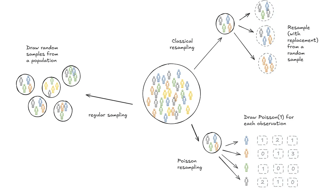
Bootstrapping is a useful technique to infer statistical features (think mean, decile, confidence intervals) of a population based on a sample collected. Implementing it at scale can be hard and in use cases with streaming data, very complicated. When trying to learn how to bootstrap at scale, I came across a Google blog (almost a decade old) that introduces Poisson bootstrapping. Since then I’ve discovered an even older paper, Hanley and MacGibbon (2006), that outlines a version of this technique. This post is an attempt to make sure I’ve understood the logic well enough to explain it to someone else. We’ll start with a description of classical bootstrapping first to motivate why Poisson bootstrapping is neat.
Classical bootstrapping
Suppose we wanted to calculate the mean age of students in a school. We could repeatedly draw samples of 100 students, calculate the means and store them. Then we could take a final mean of those sample means. This final mean is an estimate of the population mean.
In practice, it’s often not possible to draw repeated samples from a population. This is where bootstrapping comes in. Bootstrapping sort of mimics this process. Instead of drawing samples from the population we draw samples (with replacement) from the one sample we collected. The psuedo-samples are referred to as resamples.
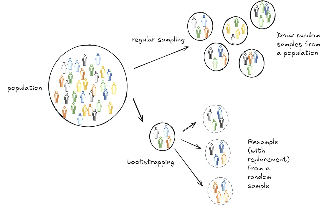
Turns out this is extremely effective. It’s more computationally expensive than a closed form solution but does not make strong assumptions about the distribution of the population. Additionally, it’s cheaper than repeating sample collections. In practice, it’s used a lot in industry because in many cases either closed form solutions don’t exist or are hard to get right—for instance, when inferring deciles of a population.
Why does bootstrapping work?
Bootstrapping feels wrong. Or at least the first time I learned about it, it didn’t feel right. Why should one sample contain so much information?
Sampling with replacement from the original sample you drew is just a way for you to mimic drawing from the population. The original sample you drew, on average, looks like your population. So when you resample from it, you’re essentially drawing samples from the same probability distribution.
What if you just happen to draw a weird sample? That’s possible and that’s why we resample. Resampling helps us learn about the distribution of the sample itself. What if you original sample is too small? As the number of observations in the sample grow, bootstrapping estimates converge to population values. However, there are no guarantees over finite samples.
There are problems but given the constraints we operate in, it is the best possible information we have on the population. We don’t have to assume the population has a specific shape. Given that computation is fairly cheap, bootstrapping becomes a very powerful tool to use.
Demonstrating classical bootstrapping
We’ll explain bootstrapping with two examples. The first is a tiny dataset where the idea is that you can do the math in your head. The second is a larger dataset for which I’ll write down code.
Example 1: Determining the mean age of students in a school
We’re tasked to determine the mean age of students in a school. We sample 5 students randomly. The idea is to use those 5 students to infer the average age of all the students in the school. This is silly (and statistically improper) but bear with me.
ages = [12, 8, 10, 15, 9]
We now sample from this list with replacement.
sample_1 = [ 8, 10,  8, 15, 12]
sample_2 = [10, 10, 12,  8, 15]
sample_3 = [10, 12,  9,  9,  9]
....
do this a 1000 times
....
sample_1000 = [ 9, 12, 12, 15,  8]
For each resample, calculate the mean.
mean_sample_1 = 10.6
mean_sample_2 = 11
mean_sample_3 = 9.8
...
mean_sample_1000 = 11.2
Take a mean of those means.
mean_over_samples=mean(mean_sample_1, mean_sample_2, .. , mean_sample_1000)
This mean then becomes your estimate of the population mean. You can do the same thing over any statistical property: Confidence intervals, deviations etc.
Example 2: Determining the 95th percentile for ‘time to process payment’
Customers on a food delivery app make payments on the app. After a payment is successful, an order is placed with the restaurant. The time to process payment calculated as the time between when a customer presses the ‘Make Payment’ button and when feedback is delivered (payment successful, payment failed) is a critical metric that reflects platform reliability. Millions of customers make payments on the app every day.
We’re tasked to estimate the 95% percentile of the distribution to be able to rapidly detect issues.
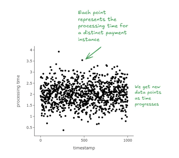
We illustrate classical bootstrapping in the following way:
- We assume that there’s some population that has a million observations. In the real world, we never observe this data.
- We randomly sample 1/10th of this population. So we take 10,000 observations. In reality this is the only data we observe.
- We then apply the same procedure we discussed above. We resample observations from our observed data with replacement. We do this many, many times.
- Each time when we resample, we calculate the 95th percentile of that distribution.
- Finally we take the mean of the 95th percentile values and find confidence intervals around it.
We get the graph below. Magically, we find that the confidence intervals we just generated contain the true 95th percentile (from our population).
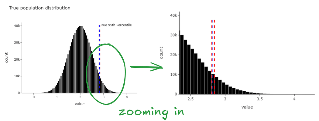
We can see the same data at the level of the bootstrapped statistic.
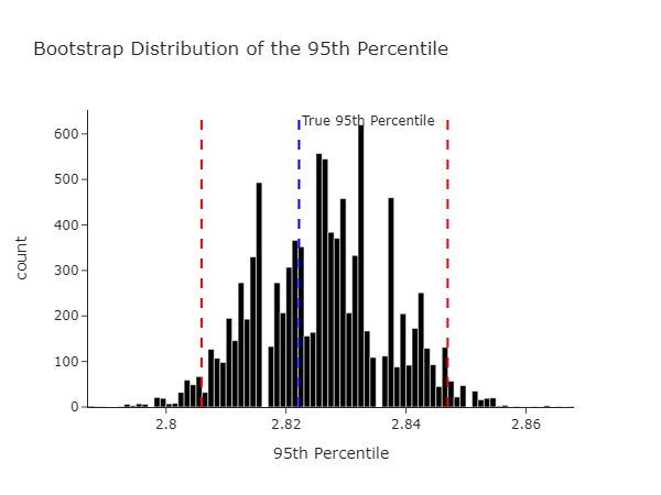
The code to generate the above is below, give it a try yourself!
def bootstrap_nth_percentile_and_ci(
    data: List[float], n_iter: int = 1000, alpha: float = 0.95, percentile: float = 95
) -> Tuple[float, float, float, float]:
    """Compute the nth percentile and confidence interval using bootstrapping

    Args:
        data (List[float]): List of data
        n_iter (int, optional): Number of bootstrap samples. Defaults to 1000.
        alpha (float, optional): Confidence level. Defaults to 0.95.
        percentile (float, optional): Percentile to compute. Defaults to 95.

    Returns:
        Tuple[float, float, float, float]: Tuple containing the percentile, mean,
        lower bound, and upper bound

    """

    n = len(data)

    bootstrap_samples = np.random.choice(data, (n_iter, n), replace=True)
    percentiles = np.percentile(bootstrap_samples, percentile, axis=1)

    mean = percentiles.mean()
    lower = np.percentile(percentiles, (1 - alpha) / 2 * 100)
    upper = np.percentile(percentiles, (1 + alpha) / 2 * 100)

    return percentiles, mean, lower, upper


# population specifics
mean_time = 2.0
std_dev = 0.5
processing_time = np.random.normal(loc=mean_time, scale=std_dev, size=1_000_000)

# sample from processing time
sample = np.random.choice(processing_time, 10000) # note we only sample 1/10th of the population

percentiles, mean, lower_bound, upper_bound = bootstrap_nth_percentile_and_ci(
    sample, n_iter=10000, percentile=95
)
This all works great, what’s next?
Now that we’ve established that classical bootstrapping actually works we’ll try and establish what’s happening from a mathematical perspective. Usually texts will just tell you to skip this part if you’re not interested. I’ll encourage you to stick around though because this is where the real fun is.
Take a break
Let’s think through a game now. Imagine you had a bag filled with 5 balls: A red, blue, yellow, green and purple ball. You need to draw 5 balls from the bag, one at a time. After you draw a ball, you put it back into the bag and then draw again. So each time you choose a ball, you have 5 differently coloured balls to choose from. After each round you record the ball that was chosen in a empty slot (as shown below).
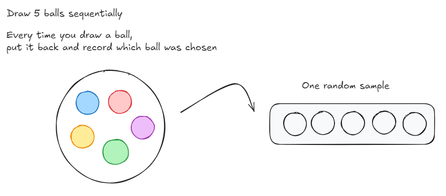
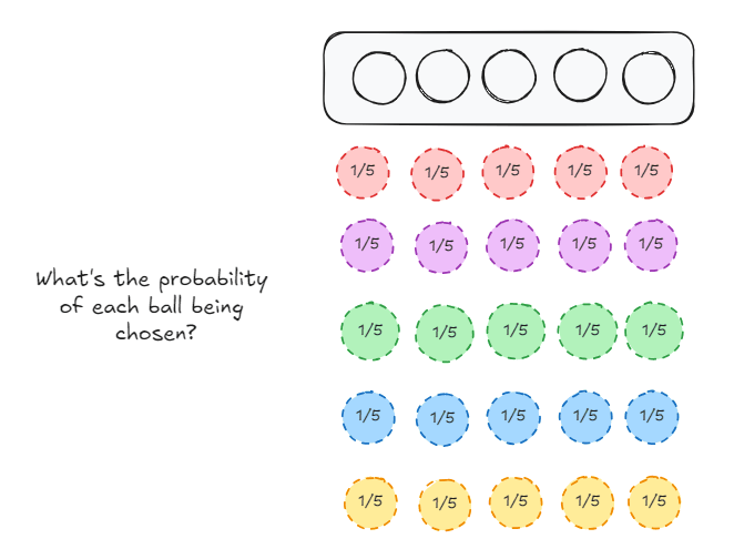
Now, if I were to ask you, what’s the probability of each ball being chosen for a each slot that we have to fill?
For slot 1,
- The red ball can be chosen with probability 1/5
- The purple ball can be chosen with probability 1/5
- The green ball can be chosen with probability 1/5
- The blue ball can be chosen with probability 1/5
- The yellow ball can be chosen with probability 1/5
The same case extends to slot 2, 3, 4 and 5
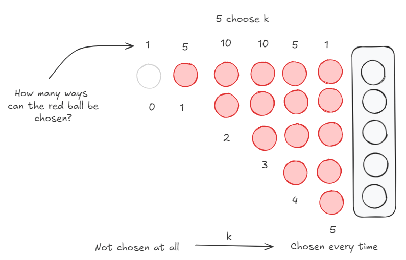
Lets focus on the red ball for a bit. It can be chosen a minimum of zero times (it isn’t chosen at all) and a maximum of 5 times. The probability distribution of the occurrence of the red ball is the following:
- Red ball chosen 0 times: This can only happen in 1 way.
- Red ball chosen 1 time: This can happen in 5 ways. Red ball is chosen for slot 1, Red ball is chosen for slot 2 … (you get the drift).
- Red ball chosen 2 times: This can happen in 10 ways. Fix the red ball on slot 1, there are 4 options. Fix the red ball on slot 2, there are 3 new options, …
- Red ball chosen 3 times: This can happen in 10 ways. This is exactly similar to the logic above.
- Red ball chosen 4 times: The can happen in 5 ways. Similar to being chosen once.
- Red ball is chosen 5 times. This can happen in 1 way.
This is just 5 choose k, where k = {0, 1, 2, 3, 4, 5}
Let’s put these two facts together just for the red balls
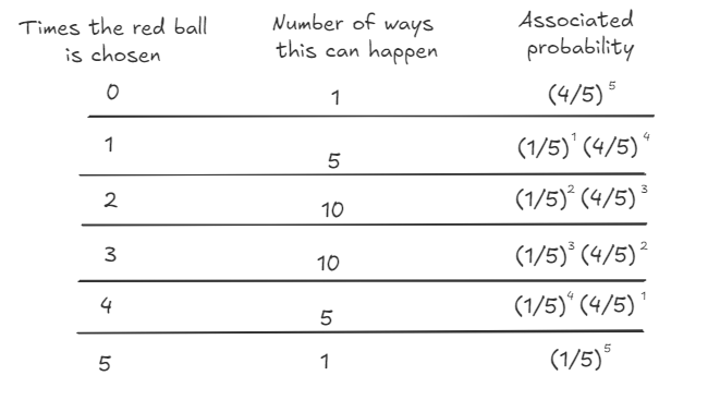
What we just described is the binomial distribution where n = 5 and p = 1/5
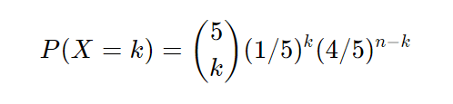
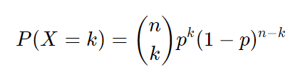
Or more generally,
Now just substitute balls for observations.
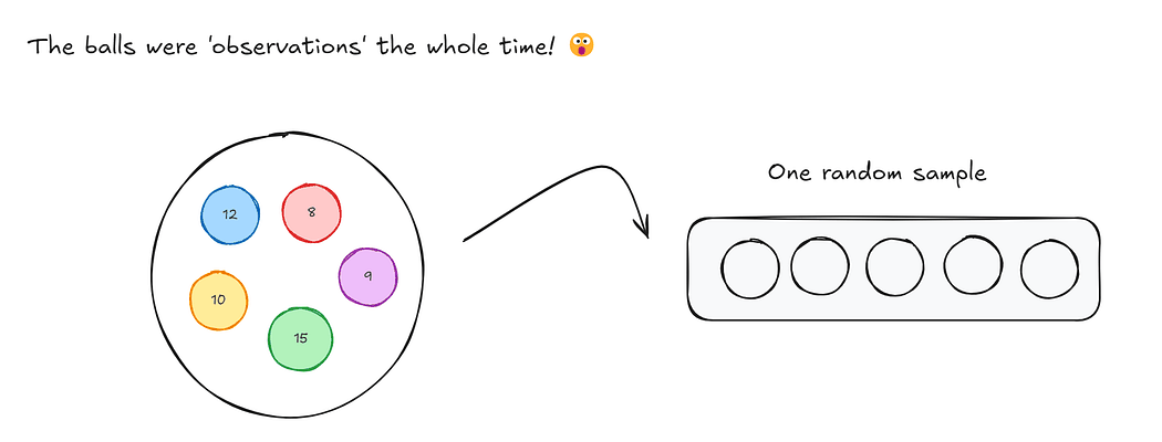
So when we bootstrap, we essentially are drawing each observation from a binomial distribution.
In classical bootstrapping, when we resample, each observation follows the binomial distribution with n = n, k = {0, …, n} and p = 1/n. This is also expressed as Binomial(n , 1/n).
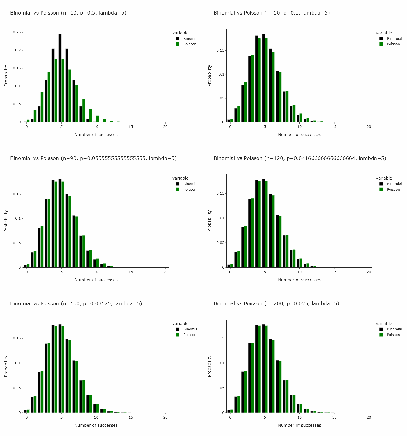
Now, a very interesting property of the binomial distribution is that as n turns larger and larger, and p turns smaller and smaller, the binomial distribution converges to a Poisson distribution with Poisson(n/p). Some day I’ll write an intuitive explanation of why this happens but for now if you’re interested, you can read this very well written piece.
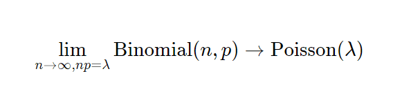
This works for any n and p such that n/p is constant. In the gif below we show this for lambda (n/p) = 5.
In our special case, we’ll just converge to Poisson(1) as p is just 1/n.
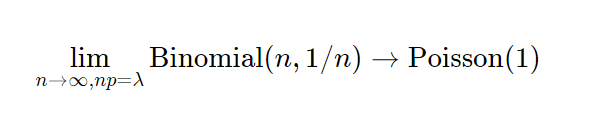
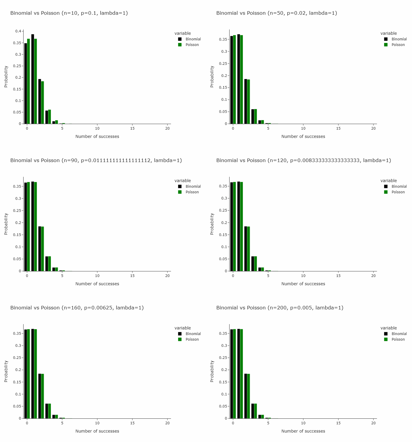
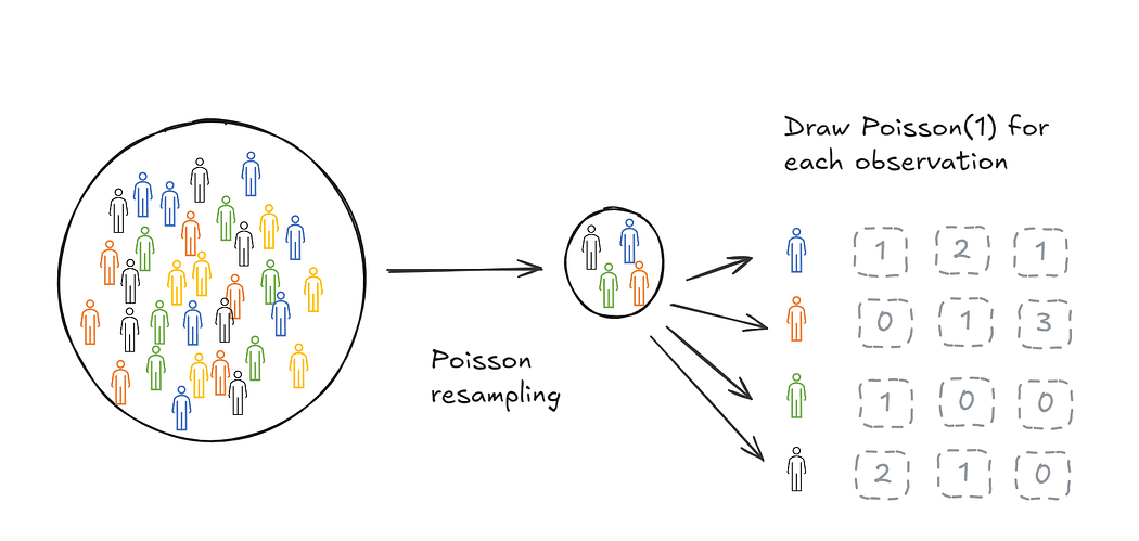
Then it follow that another way to resample would be to draw each observation from a Poisson(1) distribution.
Poisson bootstrapping means that we use a Poisson(1) process to generate resamples for bootstrapping a statistic.
Big deal, why is this useful?
There are two stages of bootstrapping a statistic of interest. The first stage is to create resamples, the second stage is to calculate the statistic on each resample. Classical and Poisson bootstrapping are identical on the second stage but different on the first stage.
There are two ways in which this is useful:
- Poisson bootstrapping reduces the number of passes we need to make over data.
- Poisson bootstrapping works in cases where we don’t have a fixed n. For instance, when we’re streaming data in.
Reducing the number of passes while resampling
The Poisson bootstrap allows for significant computation gains while creating resamples. The best way to look at this is in code.
def poisson_bootstrap_nth_percentile_and_ci(
    data: List[float], n_iter: int = 1000, alpha: float = 0.95, percentile: float = 95
) -> Tuple[float, float, float, float]:

    data = np.array(data)
    n = len(data)

    weights = np.random.poisson(1, (n_iter, n))

    percentiles = []

    for weight in weights:
        resampled_data = np.repeat(data, weight)
        percentile = np.percentile(resampled_data, 95)
        percentiles.append(percentile)

    mean_percentile = np.mean(percentiles)
    lower_bound = np.percentile(percentiles, (1 - alpha) / 2 * 100)
    upper_bound = np.percentile(percentiles, (1 + alpha) / 2 * 100)

    return percentiles, mean_percentile, lower_bound, upper_bound
Compare line (8) above, with the equivalent line in the classical bootstrap:
# classical, needs to know (data)
bootstrap_samples = np.random.choice(data, (n_iter, n), replace=True)

# poisson, does not need to know (data)
weights = np.random.poisson(1, (n_iter, n))
In the classical bootstrap, you need to know data, while in the Poisson bootstrap you don’t.
The implications for this are very significant for cases where data is very large (think 100s of millions of observations). This is because mathematically, generating resamples reduces to generating counts for each observation.
- In classical bootstrapping, the counts for each observation follow a Binomial(n, 1/n). Together they follow a Multinomial(n, 1/n, 1/n, …, 1/n). This means when you generate a count for an observation, this impacts the count for the other observations. For instance, in our ball example, once you’ve generated the count for a red ball, this has a direct impact on the counts for the other balls. For instance, if the count for the red ball is 2, then we know that we only have 3 more balls we can choose.
- In Poisson bootstrapping, the counts for each observation are independent on each other. So if you need 1000 resamples, you just generate 1000 Poisson(1) draws for the red ball. Then you’re done and you can move on to the next observation.
Resampling when n is unknown
There are cases where n is effectively unknown. For instance, in cases where you’re streaming in payment data or where data is so large that is lives across multiple storage instances.
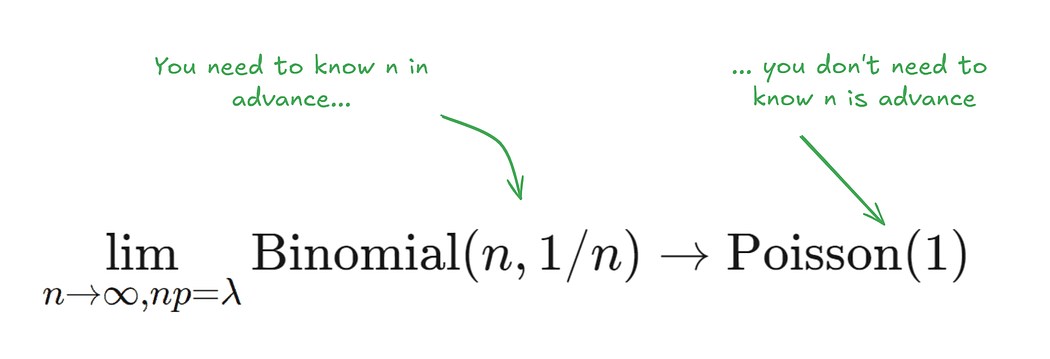
In classical bootstrapping every time we observe an increased n, we have to redo the resampling process again (as we sample with replacement). This renders this method quite computationally expensive and wasteful. In the Poisson bootstrap we can just save our Poisson(1) draws for each instance. Every time a new instance is added all we need to do is to generate the Poisson(1) draws for this new instance.
Conclusion
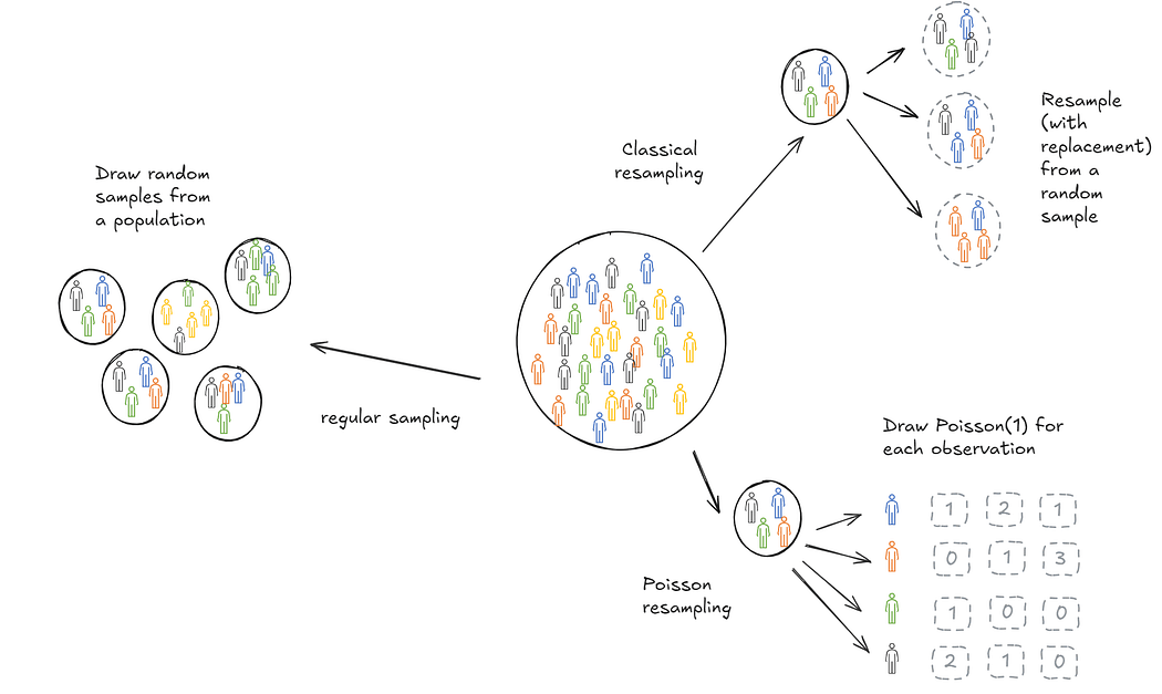
Classical bootstrapping is a very effective technique for learning the distribution of a statistic from a sample collected. In practice, it can be prohibitively expensive for very large datasets. Poisson bootstrapping is a version of bootstrapping that enables efficient parallel computation of resamples. This is because of two reasons:
- Resampling under Poisson bootstraps means we only make one pass over each observation.
- In streaming data cases, Poisson bootstraps allow us to process new resamples incrementally rather than having to resample over the entire dataset in one go.